News

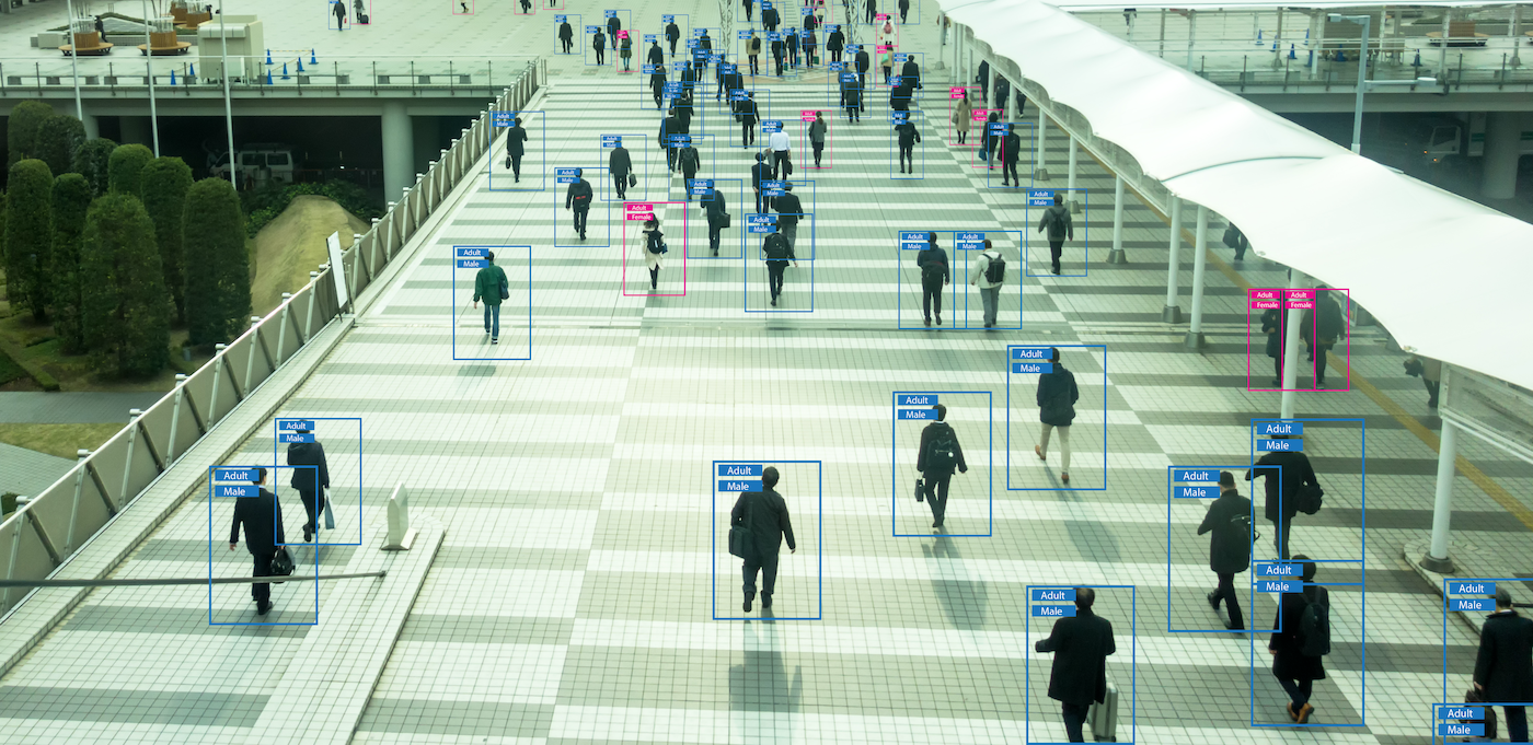
Real-Time Object Detection – Xilinx Vitis AI

• TECHNOLOGY
• 20 Jul

Xilinx has recently released its brand new machine learning development kit – Vitis AI. We had the opportunity to explore its AI development environment and the tool flow. In this blog, we like to provide readers a clear understanding of how to develop a real-time object detection system on one of the Xilinx embedded targets. We will use the VGG based Single Shot Detector (SSD) model for the detection application. Since our audience comes from various domains and has varying working experience with Deep Learning as well as Xilinx devices, we would like to start with the basics. So, we are not going to train a model from scratch but will cover the workflow from the Machine learning framework model to the one able to deploy on Xilinx- Zynq UltraScale+ MPSoC ZCU104.

Environment Setup and Installation.

For the Machine learning model development, we are using the Caffe framework. I know, a lot of readers might ask why Caffe, it’s old and why not Tensorflow. Yes you are right, Caffe is old, but there are people still out there use it like Xilinx and we thought it will be nice for beginners to understand the ML concepts with ease. But, don’t worry we will cover a working example with Tensorflow in the next blog post.

Note: The tutorial is based on Vitis AI 1.1.

Host Setup

So let’s discuss how we can set up Caffe and is it difficult? No, it’s pretty easy with the new Vitis AI 1.1 as it provides Caffe preinstalled on the Docker package which is available at https://github.com/Xilinx/Vitis-AI. On this page, you will find all the details for setting up Vitis AI on your host PC (Ubuntu 18.04 in our case). We encourage advanced users to install GPU enabled docker container as it would fasten the quantization tool flow.

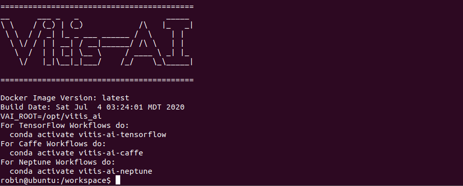
At this point, the environment is set up and Caffe conda environment can be instantiated with the following command

robin@ubuntu:/workspace$ conda activate vitis-ai-caffe

Now your terminal will output something similar as follows:

(vitis-ai-caffe) robin@ubuntu:/workspace$

Setting Up the Host (Using VART)

The Vitis AI runtime enables applications to use the unified high-level runtime API for both cloud and edge. Therefore, making cloud-to-edge deployments seamless and efficient. The procedure for installing the cross-compilation system and setting up the glob library is clearly explained here: https://github.com/Xilinx/Vitis-AI/tree/master/VART.

Finally, you will be able to cross-compile a sample, take resnet50 as an example.

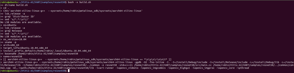
If there are no errors, then VART is successfully installed in the Host PC.

Setting Up Vitis AI Library

The Vitis AI Library is a set of high-level libraries and APIs built for efficient AI inference with the Deep-Learning Processor Unit (DPU). It is built based on the Vitis AI Runtime with Unified APIs, and it fully supports XRT 2019.2. They encapsulate a lot of high quality and efficient neural networks, which simplifies the use of deep learning neural networks without the knowledge of deep learning or FPGAs.

Please follow the instruction for setting up the Host PC with theVitis AI library on the following page: https://github.com/Xilinx/Vitis-AI/tree/master/Vitis-AI-Library If you have done the VART setup, then you don’t need to do any further installations but make sure you are able to compile some sample from Vitis AI Library.

Evaluation Board Setup

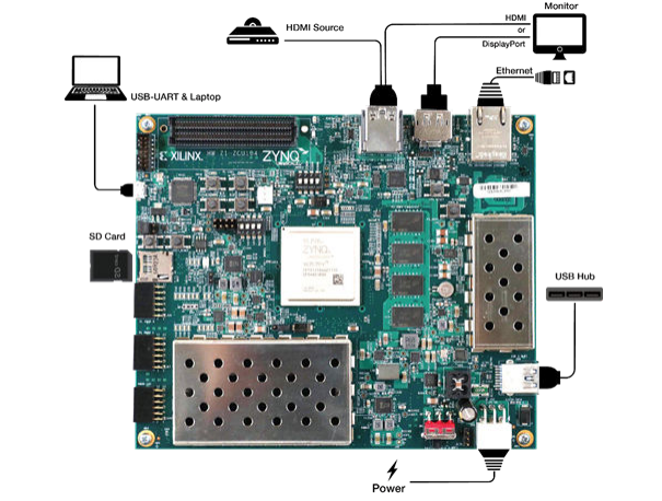
The Xilinx ZCU104 evaluation board uses the mid-range Zynq UltraScale+ device to enable you to jumpstart your machine learning applications. For more information on the ZCU104 board, see the Xilinx website: https://www.xilinx.com/products/boards-and-kits/zcu104.html. The main connectivity interfaces for ZCU104 are shown in the following figure.

The first step is to download the demo Linux image with Vitis AI DPU enabled from here.

It is highly recommended to run the power management patch by running irps5401 to avoid power off or system hangs while running the samples. If you cant find this command in the prebuilt image, please download the updated image from here: https://www.xilinx.com/bin/public/openDownload?filename=xilinx-zcu104-dpu-v2019.2-v2.img.gz.

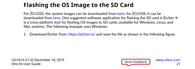
We encourage the readers to go through all the procedures (page no: 20 – 30) for setting up the ZCU104 board in the Vitis AI user guide: https://www.xilinx.com/support/documentation/sw_manuals/vitis_ai/1_0/ug1414-vitis-ai.pdf.

While following the above resource, please make sure, you install the required packages for both VART and Vitis AI Library. The user guide has only mentioned the VART installation, but you can find the Vitis Library installation for the board here: https://github.com/Xilinx/Vitis-AI/tree/master/Vitis-AI-Library

VART Installation Check

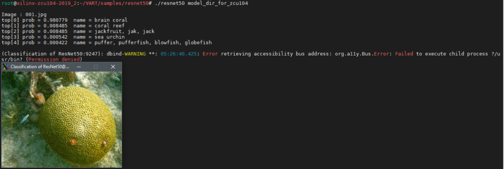
It is very important to check the VART installation on the target board. On your target board, change the directory where VART samples were downloaded.

#cd ~/VART/samples/resnet50

Run the example.

#./resnet50 model_dir_for_zcu104

If the above executable program does not exist, run the following command to compile and generate the corresponding executable program.

#bash -x build.sh

Vitis AI library check

Since we will be leveraging the power of Vitis AI Library for certain pre and post-processing steps while doing the inference, it is great to do some prebuilt samples provided by the Vitis AI library. If you have followed the above-mentioned procedure for installing the AI model packet for the target board. Then all the models will be stored under /usr/share/vitis_ai_library/models/. Each model is stored in a separate folder that is composed of.

• [model_name].elf
• [model_name].prototxt
• meta.json

we will see what are all these files while discussing object detection, stay tuned!!!. So let’s run some examples to check the installation. We will run the face detection example and we will use the dense_640_360.elf model. Go to your terminal and type

#cd /usr/share/vitis_ai_library/models/

#cp -r dense_640_360/ ~/overview/samples/facedetect/

Build the executable.

#sh -x build.sh

Run the demo on a single image

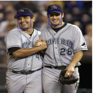
#./test_jpeg_facedetect densebox_640_360 sample_facedetect.jpg

Here is the output. I know the model didn’t detect one of those faces. Since the model is pre-trained and compiled by Xilinx, we cannot make a conclusion about why the model does that and it is out of the scope of this blog.

Now we have successfully set up the environment(Host and target) for the further development steps

Object Detection on ZCU104

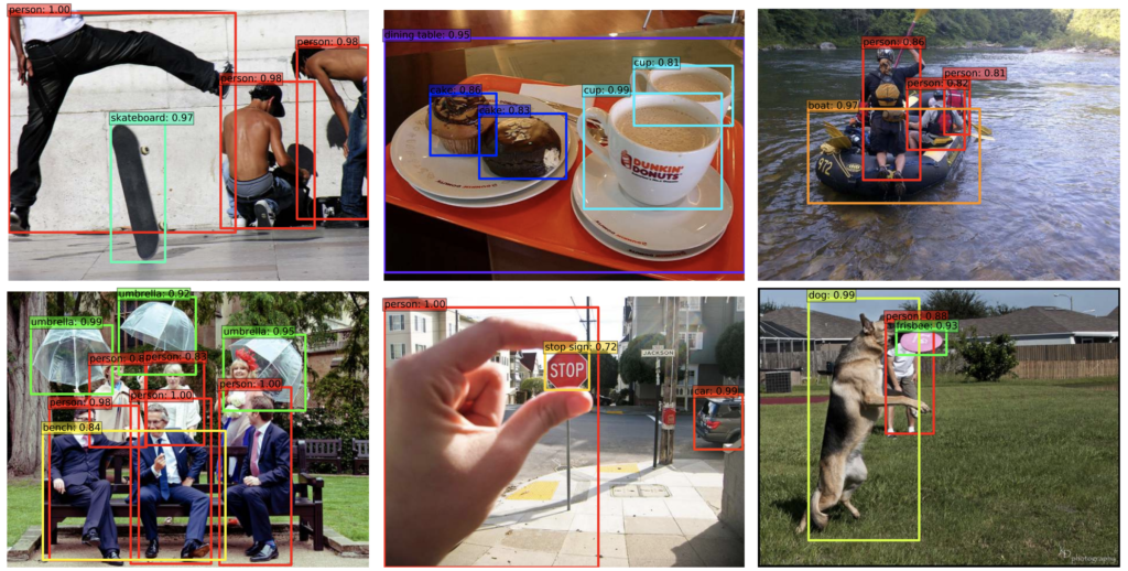
Object detection is one of the important areas of Computer vision where a lot of research has been going on. We strongly urge our readers first to get a clear understanding between the various computer vision tasks namely, Image classification, detection, and Segmentation. Image classification task assigns a class label to corresponding objects in an image, whereas in object detection, we draw a bounding box around each object of our interest and label them as we do in the classification task. if you want to get a gentle introduction for all these tasks please visit this excellent blog from famous Jason Brownlee: https://machinelearningmastery.com/object-recognition-with-deep-learning/

A few examples to illustrate the idea.

Single Shot Object detection

The Single Shot Object Detection (SSD) framework was first described by Christian Szegedy et all in the paper titled SSD: Single Shot MultiBox Detector. For object detection, we have mainly two types of detectors Multistage state of the art detectors like the RCNN family RCNN, Faster RCNN, etc. and Single-stage detectors such as Yolo and SSD. Comparing to the RCNN models, Single-stage detectors are faster, thus making them suitable for Real-time Object detection. Since SSD uses multi-scale convolutional features at the top of the network instead of a fully connected layer in Yolo makes them faster and more accurate. Please see the comparison between these networks for speed and accuracy.

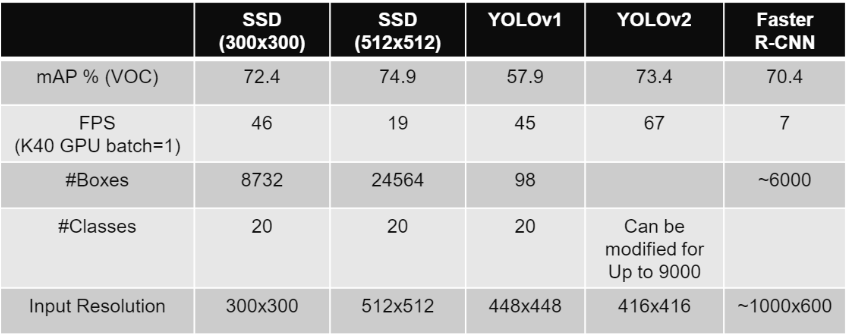
As you have noticed SSD comes in different formats, which depends on the size of the input image. In the above comparison, we have used VGG16 as the feature extractor, and as opposed to the real work, input image dimensions are $300 \times 300$. We highly recommend the audience to get an intuitive idea of How exactly SSD detects objects from the input image. Please visit this excellent tutorial by Sagar Vinodbabu on a-PyTorch-Tutorial-to-Object-Detection.

Hopefully, Now we understand how SSD works at least the workflow. For the rest of the blog steps, we will be providing associated files for those who want to implement themselves. This will help you how to invoke the Vitis AI tools for accelerating.

Note: If you have installed the Vitis AI docker runtime system on your host, A workspace folder will be created in the docker runtime system. Please copy our associated file’s root folder to \workspace.

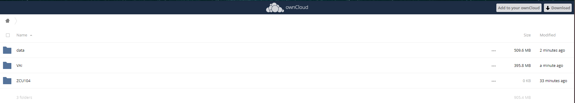
Files description :

1. VAI: Contains the files for quantizing and compiling your Caffe pre-trained model.
   • “float.prototxt”: used for quantizing/compiling the models for deployment on the target hardware. Note: Please take care of the path specified for calibration data and text files so they point to the correct location. if you are directly following the tutorial no changes has to be made.
   • “float.caffemodel” : pretrained weights.
   • “quantize_and_compile.sh”: script for automating the quantization and compilation of our moel. We will examine it in a bit detail soon.
2. data: Here we have all the files associated with training data like calibration data, text files, label maps, etc. which are required by the “float.prototxt” file while quantizing the network.
3. ZCU104: contains the files for deploying the compiled model on the target board.

Now we can quantize the model with Vitis AI quantizer and compile using AI Compiler. You can run these tools by running the following command (you may need to make the file executable first)

/workspace/SSD$ cd VAI

/workspace/SSD/VAI$ ./quantize_and_compile.sh

Open the script, if you need to make any changes like GPU ID setting etc. I have been testing with a CPU only machine. For faster quantization, use GPU enabled devices.

#!/usr/bin/env bash
#uncomment for GPU usage
#export GPUID=0
net=vgg16_ssd

#working directory
work_dir=$(pwd)
#path of float model
model_dir=quantize
#output directory
output_dir=compile

echo "quantizing network: $(pwd)/float.prototxt"
vai_q_caffe quantize          \
          -model $(pwd)/float.prototxt     \
          -weights $(pwd)/float.caffemodel \
          -calib_iter 100 \
          -output_dir ${model_dir} 2>&1 | tee ${model_dir}/quantize.txt

echo "Compiling network: ${net}"

vai_c_caffe   --prototxt=${model_dir}/deploy.prototxt \
        --caffemodel=${model_dir}/deploy.caffemodel \
        --output_dir=${output_dir} \
        --net_name=${net} \
        --options "{'mode':'normal'}" \
        --arch=/opt/vitis_ai/compiler/arch/dpuv2/ZCU104/ZCU104.json 2>&1 | tee ${output_dir}/compile.txt

The script runs the quantizer on your float model by running the vai_q_caffe command and you can find a sample output vai_q_caffe log file from my console for reference. After quantizing we will get the “deploy.model” and “deploy.prototxt” files required by the compilation process that are stored here. AI quantizer gives you the opportunity to test the quantized model’s accuracy and provides corresponding model files that can be used for further tuning.

Finally, the vai_c_caffe command invokes the Vitis AI compiler and compiles our quantized model to produce a dpu compatible model file called “dpu_vgg_16_ssd.elf”. For reference, vai_c_caffe log file is added too. You should be able to see something similar to these log files. We will be using the “elf” file generated for producing the inference on ZCU104.

Running the SSD model on ZCU104

Now we can deploy our SSD based object detection on the ZCU104 board. To make this process easy and faster you can find all the required files in this folder ZCU104. We will be leveraging the power of Vitis AI library for the preprocessing, model deployment, and post-process steps like bounding box decoding, apply non-max suppression, etc. We urge ambitious readers to get into the details of the Vitis AI library, where most of its components are open source and can be found here. The application sub-directory includes the following files and folders.

• dpu_vgg16_ssd: This directory contains the compiled elf model and other additional files required by the Vitis AI library for deploying the model. If you are using custom models, please copy the compiled files into this directory.”vgg16_ssd. prototxt” file provides the parameters of the detection model and the meta.json file is the configuration file of the model. The application will get the model info through this configuration file.
• vgg16_ssd.prototxt: This config prototxt file holds the pre and post-processing information related to the model. If you find any difficulties in understanding the parameters especially the prior_box_param, be free to explore the model prototxt file or the deploy. prototxt files to extract these params.
• build.sh: script to build the inference application.
• test_video_ssd.cpp: This application deploys the compiled model using the Vitis AI library and enables the user to test it with a webcam or video recording.
• process_result.hpp: Here we draw the bounding boxes over the detections.

Now copy this ZCU104 application directory to your ZCU104 board through an ethernet connection. The next step requires the Vitis AI packages and tools installed on your board if you haven’t please refer to the previous sections for setting up the target board.

Now on the board,

root@xilinx-zcu104-2019_2:~# cd ZCU104/

root@xilinx-zcu104-2019_2:~/ZCU104# sh -x build.sh

Once the build is finished, you can run the application for a webcam or video recording along by mentioning the number of threads(t) as follows

for USB cam ./test_video_ssd dpu_vgg16_ssd -t 6 0

for video file ./test_video_ssd dpu_vgg16_ssd -t 6 /path/to/video_file

Conclusion

So far, we have described the various features of the Vitis AI development environment and its tool flow. Though we haven’t covered much of machine learning concepts, this tutorial will be a great starting point for all those who want to kick start their machine learning inference application on Xilinx edge devices. We have shown the workflow from a Machine learning framework point of view and how to utilize the Vitis AI tools for developing an accelerated application. There are a lot of many samples as well as demos available in the Vitis AI GitHub page for helping readers to get acquainted with new tools along with their deep learning applications. We will be posting new tutorials with different examples in the near future until then stay tuned.